Predictin Jewelry Prices using Linear Regression

Introduction
This project’s idea hit me when I was thinking: Wouldn’t it be amazing to automate the role of jewelers or at least some of their functions? I mean, imagine having a robot or a system such that given a set of features of jewelry piece specifications, it can approximate its market value. I figured, why not build a Machine Learning model that can predict the prices of jewelry pieces given their characteristics.
Hypothesis
It’s commonly known that jewelry prices are correlated with their weight, purity, and the characteristics of the stones if included. Therefore, I believe that a Linear regression model can perform well under these circumstances where the predicted value is continuous in nature and some of the features as well.
Methodology
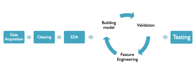 Figure 1- Development Phases
The approach I have followed throughout developing this solution is illustrated in the Figure 1. It starts by a process for acquiring and building the dataset. The collected dataset is then cleaned using multiple techniques that is to be discussed in detail in the following sections. The exploratory data analysis phase starts before building the first model to explore the data, relationships, and its nature. After that, you can see a sign of iterative process, the first iteration of this stage represents the baseline model. The remaining iterations represents multiple trials of feature engineering, model building, and validation that stops once we optimize the model as much as we can. After choosing the best model, we run it into testing to measure its performance on unseen data.
Data acquisition
I started the process by gathering data from Malabar gold and diamonds website. I used web scraping tools including Selenium and BeatifulSoup to scrape the products features and prices. Like most of the online shopping websites, Malabar’s website doesn’t render all products applicable to the filtering criteria to minimize the page load time. It loads a small batch from the whole dataset of products, if the user decides that he/she is interested he/she will scroll down the page and wait a few seconds for the website to load the next batch of data. This implementation of data rendering made it impossible for me to scrape the data with BeatifulSoup. Therefore, I had to go for Selenium to simulate the human interaction of scrolling down the page, wait a few seconds for the page load time to finish, scroll down the page again and hit the “ Show more ” button if seen. This process was repeated until the whole data is loaded and all products are rendered in the HTML page (See GIF 1). The remaining web scraping functionalities which are accessing each product page and extracting its features were handled by BeautifulSoup perfectly.
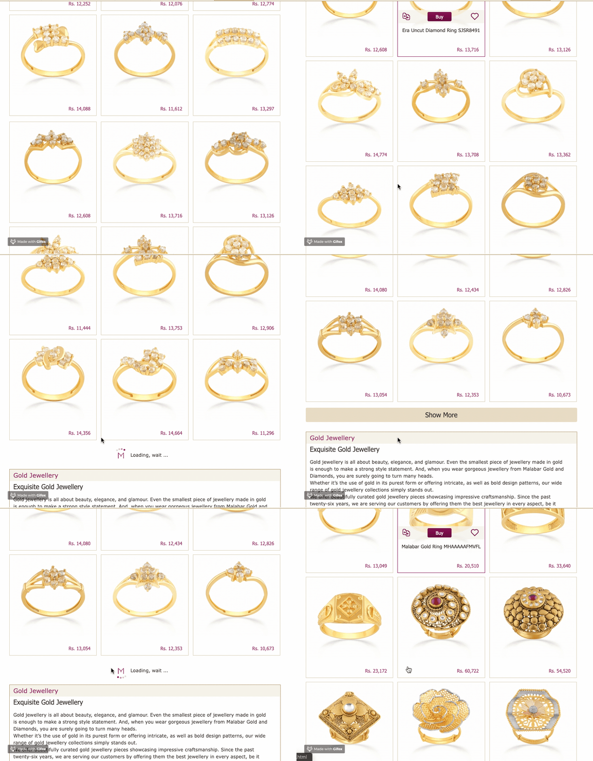 GIF 1- Load Page Demo
Data cleaning
This stage has come to prepare the data for analysis and modeling with the following steps.
- Remove non-numerical characters from price values: If you look at how the price values are stored in the dataset at the price_before_cleaning column, you can see that it contains the currency value and the string “(Approx)”. These strings shouldn’t be fed into our Machine Learning algorithm during the learning stage. Therefore, in this step, I have stored only the cost itself into the dataset. The result of this step is reflected on the price column in the Figure 2.
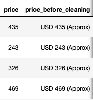 Figure 2- Price Column Cleaning
-
Convert non-numerical dimensions into numeric: Because the data was acquired via scraping a website, we have it in a textual format. This step transforms the columns datatypes into numerical datatype to feed the dataset into the linear regression in a suitable format.
-
Handle missing values: handling the missing values procedure was applied on two dimensions: records-wise and features-wise. Columns which had the majority of its entries empty (e.g., ring_size column) were discarded. Nevertheless, rows which had the majority of its columns empty due to perhaps internet connection issues or scraping issues in general were also discarded from the dataset.
-
Detecting and handling outliers.
 Figure 3- Dataset After Initial Cleaning
EDA
At first, I started by exploring the correlation and the nature of the relationship between the features against the target, and features against other features using the heatmap graph.
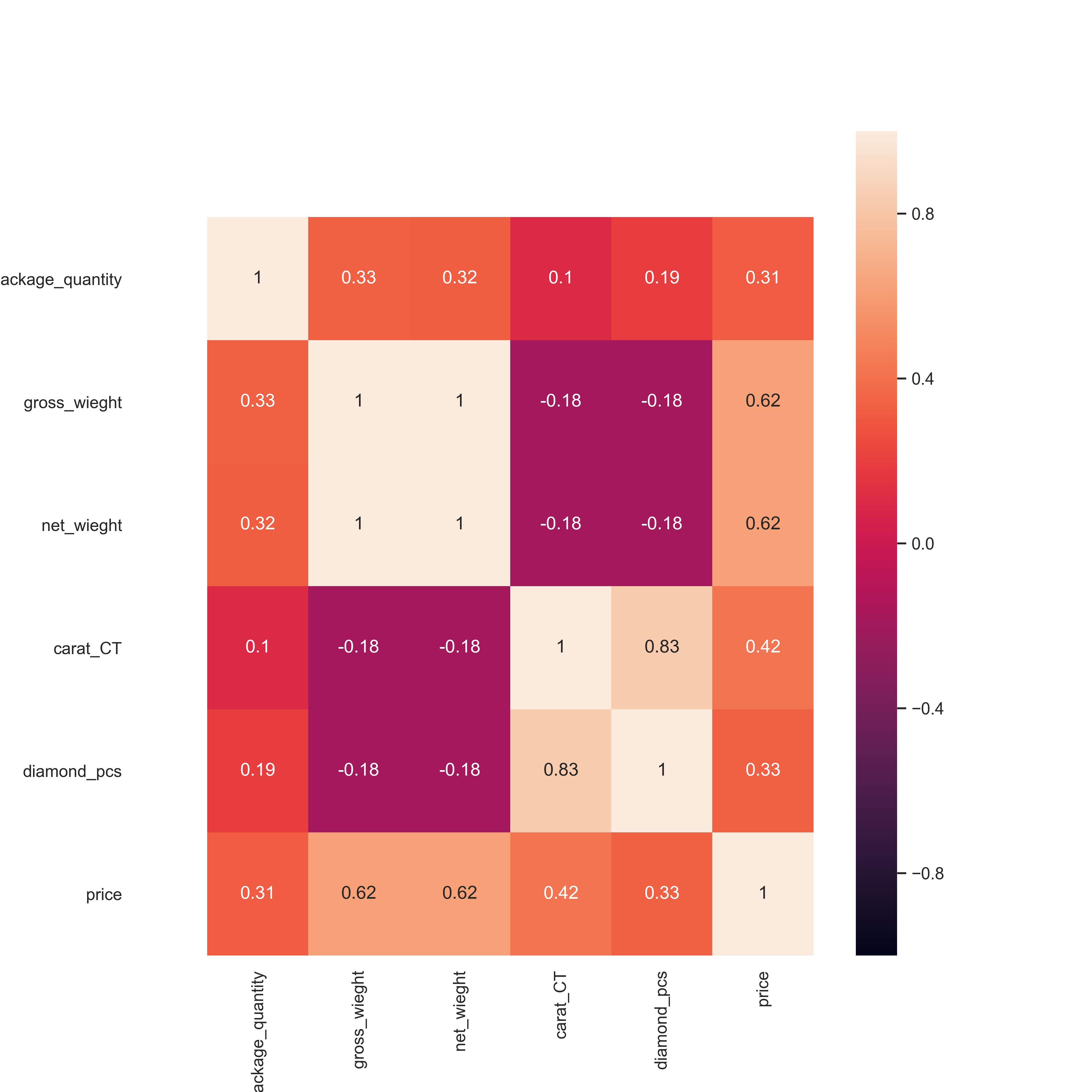 Figure 4- Baseline Heatmap
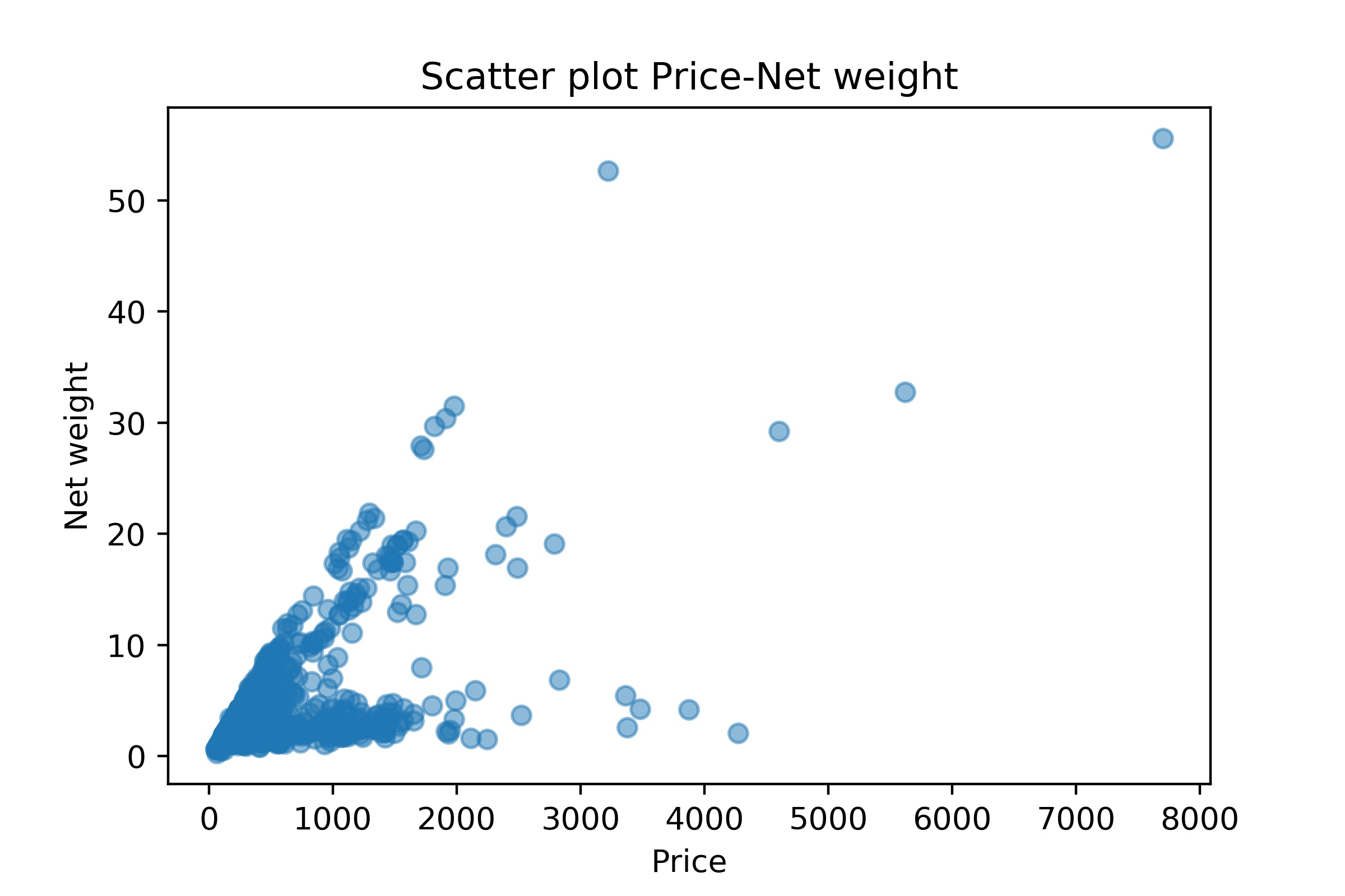 Figure 5- Scatter Plot Net Weight Against Price
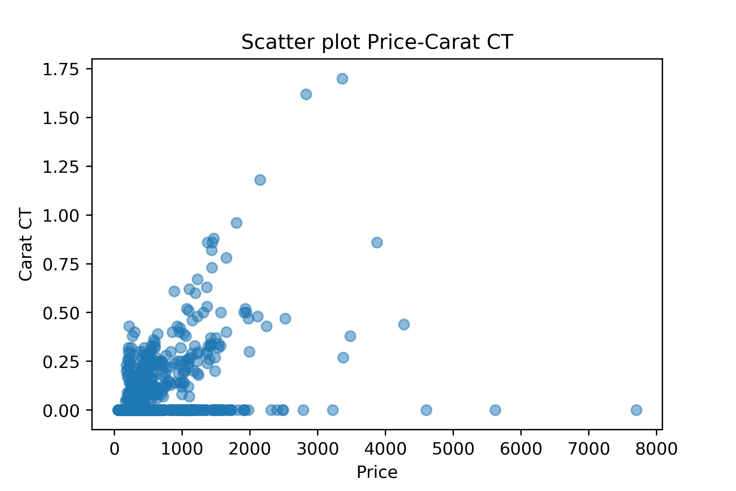 Figure 6- Scatter Plot Carat CT Against Price
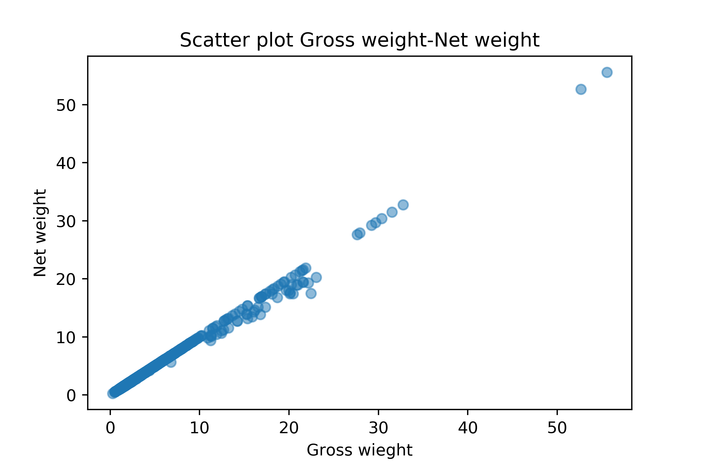 Figure 7- Scatter Plot Net Weight Against Gross Weight
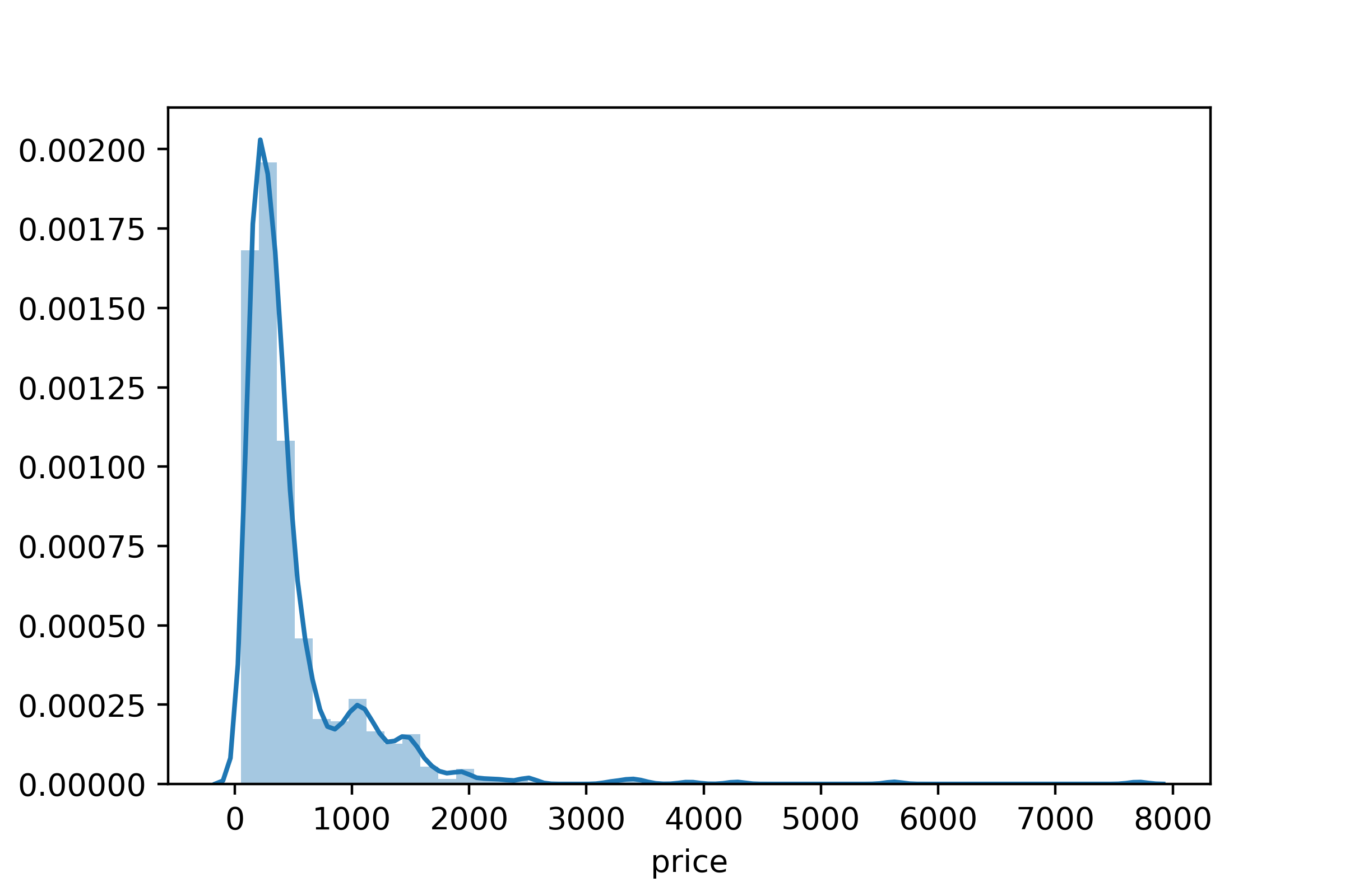 Figure 8- Distribution Plot of the Target (Price)
Looking at the heatmap, scatter plots, target distribution plot, and the box plot, I have reached the following conclusions:
- Gross weight and net weight have a highly correlated linear relationship. Therefore, one of them must be eliminated (most likely the gross weight). See Figure 3 and 6.
- Net weight has a high correlation with the target.
- Carat (CT) has a correlation with the target.
- It is obvious that the target (price) has a positively skewed distribution. One way to solve this problem is by applying a log transformation on it to get it close to a normally distributed graph (See Figure 7).
First Iteration (Baseline Model)
The baseline model used the basic features (numerical ones) scraped from the website to train itself and build its predictive model. These features are:
- Item package quantity
- Gross weight
- Net weight
- Carat CT
- Diamond pcs
Performance
Training Score: 0.6759
Validation Score: 0.6321
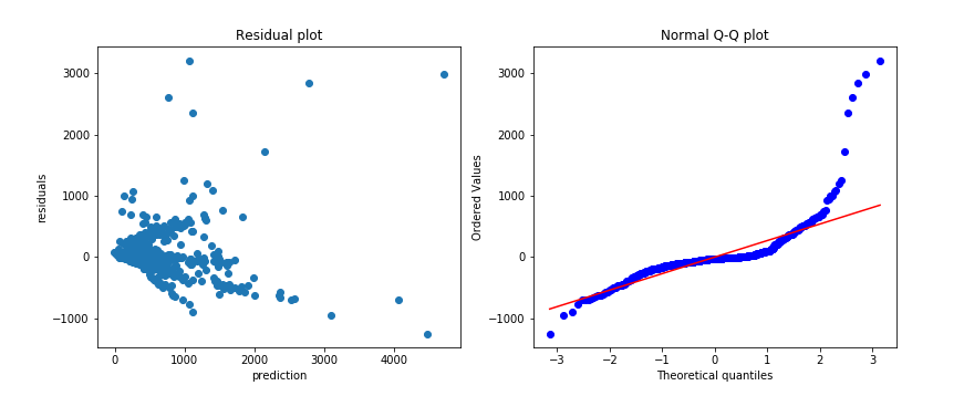 Figure 9- Residual and Q-Q plots For Baseline Model
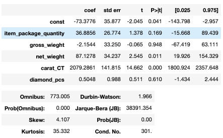 Figure 10- Baseline Model Summary
Results discussion
The training and validation scores show a good overfitting potential, most of the p-values are high, the skewness measure tells me that the shape is far from being normally distributed, and the residual plot is not showing a good random distribution.
Experimentations
From the baseline model results discussion and my conclusions at the end of the EDA phase, you could see the need and the possible potential of building a more optimized model. At this point, I started an iterative process of feature engineering, building a new version of Linear Regression model, and recording the training and validation score to compare the performance of the models and reach the most optimized one.
Optimized model
The final model used some of the numerical features and some of the categorical features after transforming them into dummy variables using one-hot encoding to fit it into a Linear Regression algorithm. The chosen features are:
- Brand_Malabar
- Purity (KT)
- Net weight
- Carat CT
- g_cert_750
- IGI_cert
Feature engineering
If you look at the three chosen features above named Brand_Malabar, g_cert_750, IGI_cert, you would realize that they did not exist in the original dataset on Figure. So, where did they come from? Each one of these features is a derived from categorical feature in the original dataset. In order to make use of categorical features in a Linear Regression model, we have to transform its unique values into dummy variables, but not necessarily all of them. To reach a decision regarding which values to keep and which to discard, I plotted a histogram for each feature that draws the count of its values. This technique helps me identify where the majority of data is clustering and use these values only as dummy variables and the rest would be discarded from the dimensions but represented using (others or neither).
- Brand_Malabar Brand is a categorical feature that represents the manufacturer of the jewelry piece. From visualizing the distribution of values at the brand dimension, I noticed that the majority of data are clustering on the Malabar and Mine brand bars. Therefore, only Malabar and Mine brands are kept as dimensions and any brand other than these two will reflect to neither.
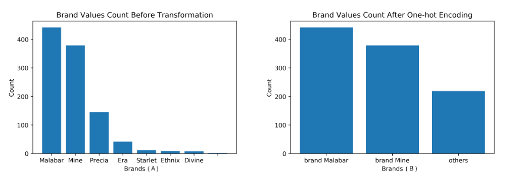 Figure 11- Brand Transformation
- g_cert_750 g_cert is a categorical feature that represents the gold certificate type. Looking at the histogram, it seemed to me it wouldn’t be fair to keep one dummy variable only due to the following reasons:
- The significantly high count belongs to items which has no certificate. Meaning it will eventually end up with the (neither) category whether it was a high or low count.
- The frequency count is not clustering at a single certificate type as much as the previous features were heavily clustering on a single feature. Therefore, for this case, I decided to include all of the unique values as dummy variables.
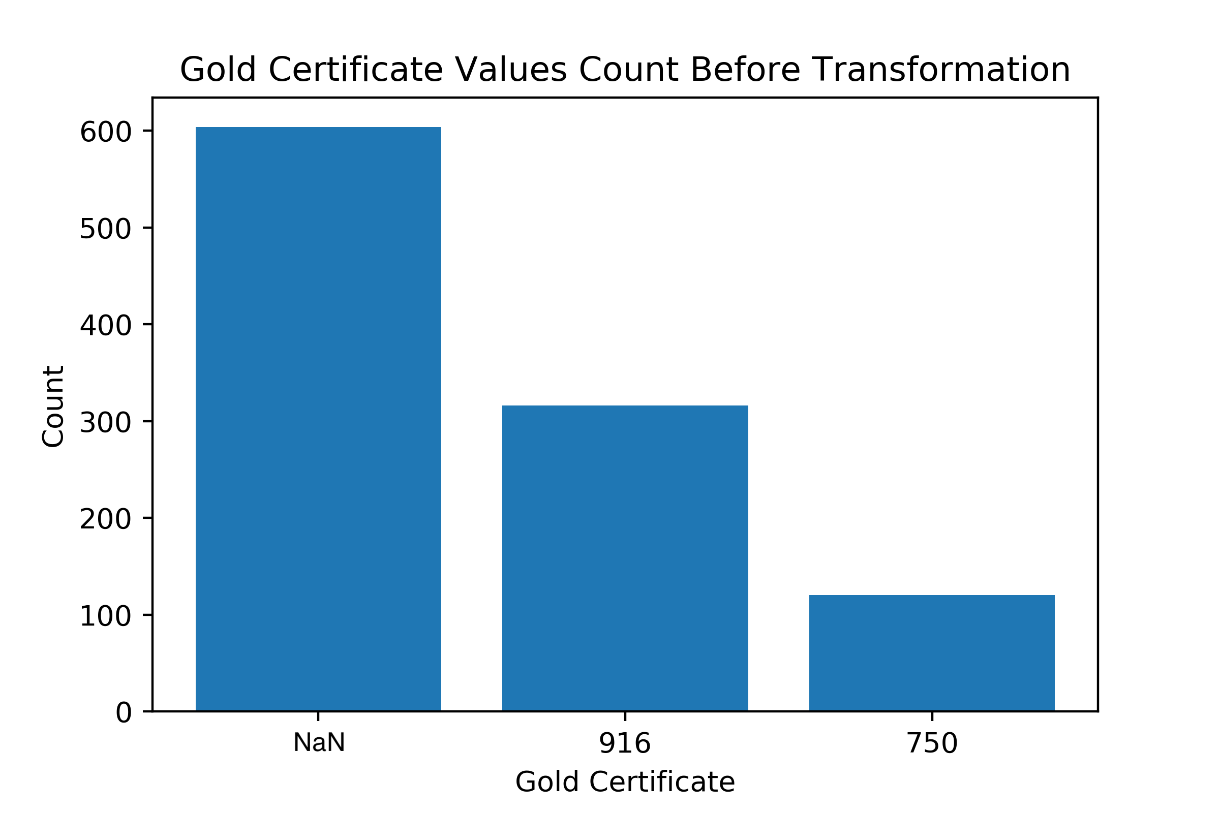 Figure 12- Gold Certificate Transformation
- IGI_cert The unique values number on this feature makes it easier to choose whether to keep all values as dummy variables or not. Since it’s binary, this limits our decision to the rule of thumb of dummy variables number. Which is { k-1 | k = len( d_cert.unique() ) }
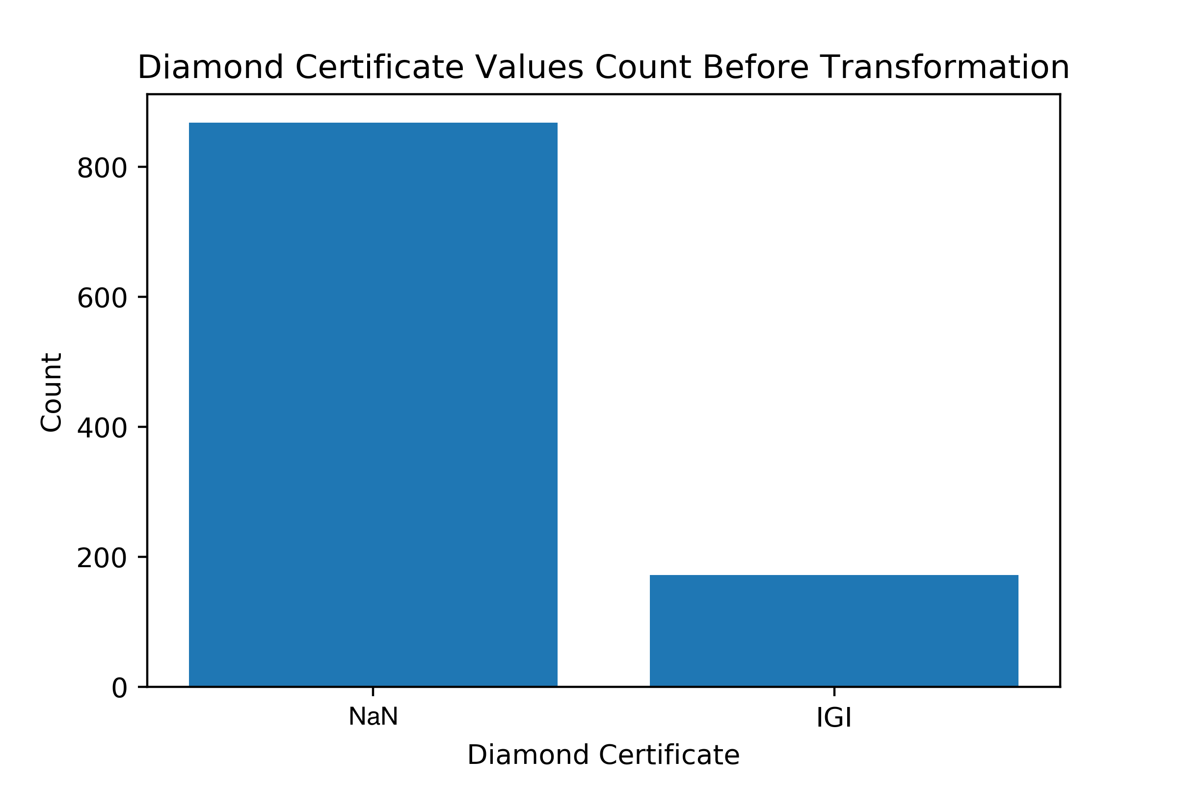 Figure 12- Diamond Certificate Transformation
Detecting and handling outliers
At the beginning, I chose to detect and handle the outliers using IQR. However, after the EDA phase and bunch of modeling experiments, I noticed that the IQR technique is eliminating point that are classified as outliers only because the dataset size is not large enough. In fact, by comparing the performance of the model with detecting and handling outliers using IQR vs. manually, the model performed better under handling it manually. Table 1 and the Figures below shows a performance comparison between the two. From the Table we see that the model which used IQR for outliers detection and handling has a higher overfitting potential than the one that filtered the dataset by setting the upper limit of price values to be 2500 $. From the model summaries we can also see from the skewness measures that model B is closer to the normal distribution than modal A is.
 Figure 13- Optimized Model Scores
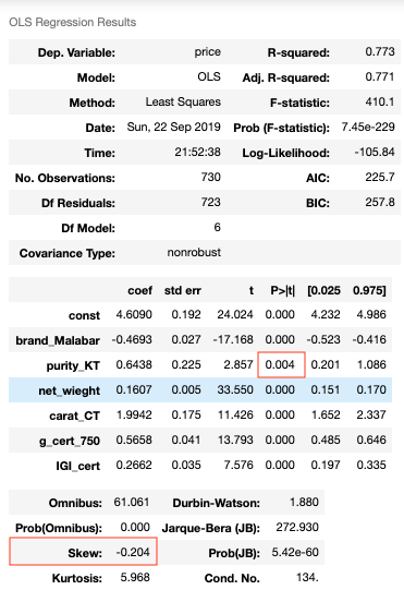 Figure 14- Model A Summary
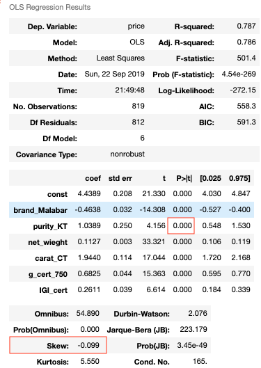 Figure 15- Model B Summary
Log transformation
I also chose to apply log transformation on the target to reduce its skewness. Figure 16 shows a distribution plot of the target after applying log transformation on it.
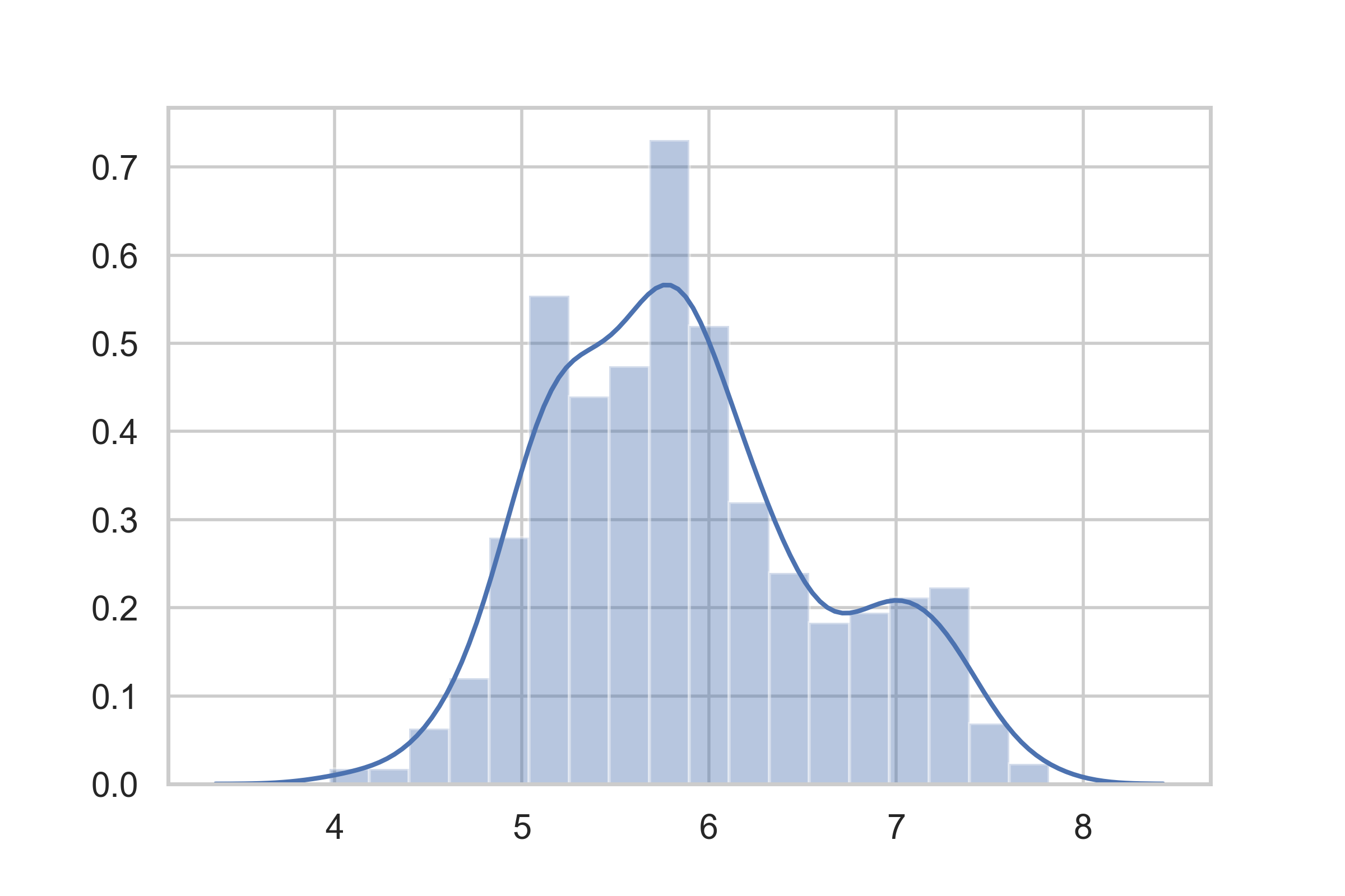 Figure 16- Distribution Plot After Log Transformation on the Target
Performance
 Figure 17- Optimized Model Scores
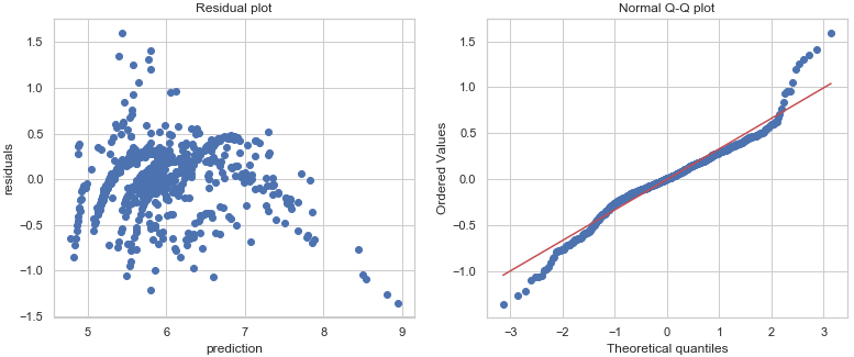 Figure 18- Residual and Q-Q plots For Optimized Model